Introduction to the ExploristicsTheme package

A custom theme and colour schemes for ggplot2.

library(ExploristicsTheme)
library(ggplot2)
library(magick)
library(magrittr)
library(scales)
library(stringr)

Usage

Theme

This package provides a theme() for use with ggplot2. It has some sensible defaults for font sizes, axis lines etc. You can add it to your plots using theme_exploristics().

## generate a plot with the Exploristics theme
cars_plot <-
  ggplot(data = mtcars, aes(x = hp, y = mpg, colour = mpg)) +
  geom_point(size = 2) +
  labs(title = "Example plot") +
  theme_exploristics()

cars_plot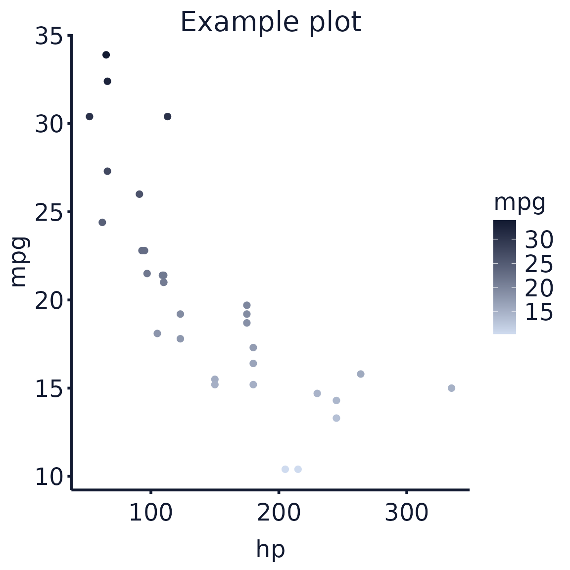

Colour and Fill

To add a colour scheme to your plot use exploristics_colour() and/or exploristics_fill().

## add colour scheme and wrap text labels
cars_plot %>%
  exploristics_colour(colour_pal = "Expl_RGB")

Text wrapper

If your plot has long titles or labels, use text_wrapper() to automatically wrap them onto a new line.

## generate a plot with a long title
cars_plot <-
  ggplot(data = mtcars, aes(x = hp, y = mpg, colour = mpg)) +
  geom_point(size = 2) +
  labs(title = "Example plot title that is a bit too long to look good without wrapping") +
  theme_exploristics()

cars_plot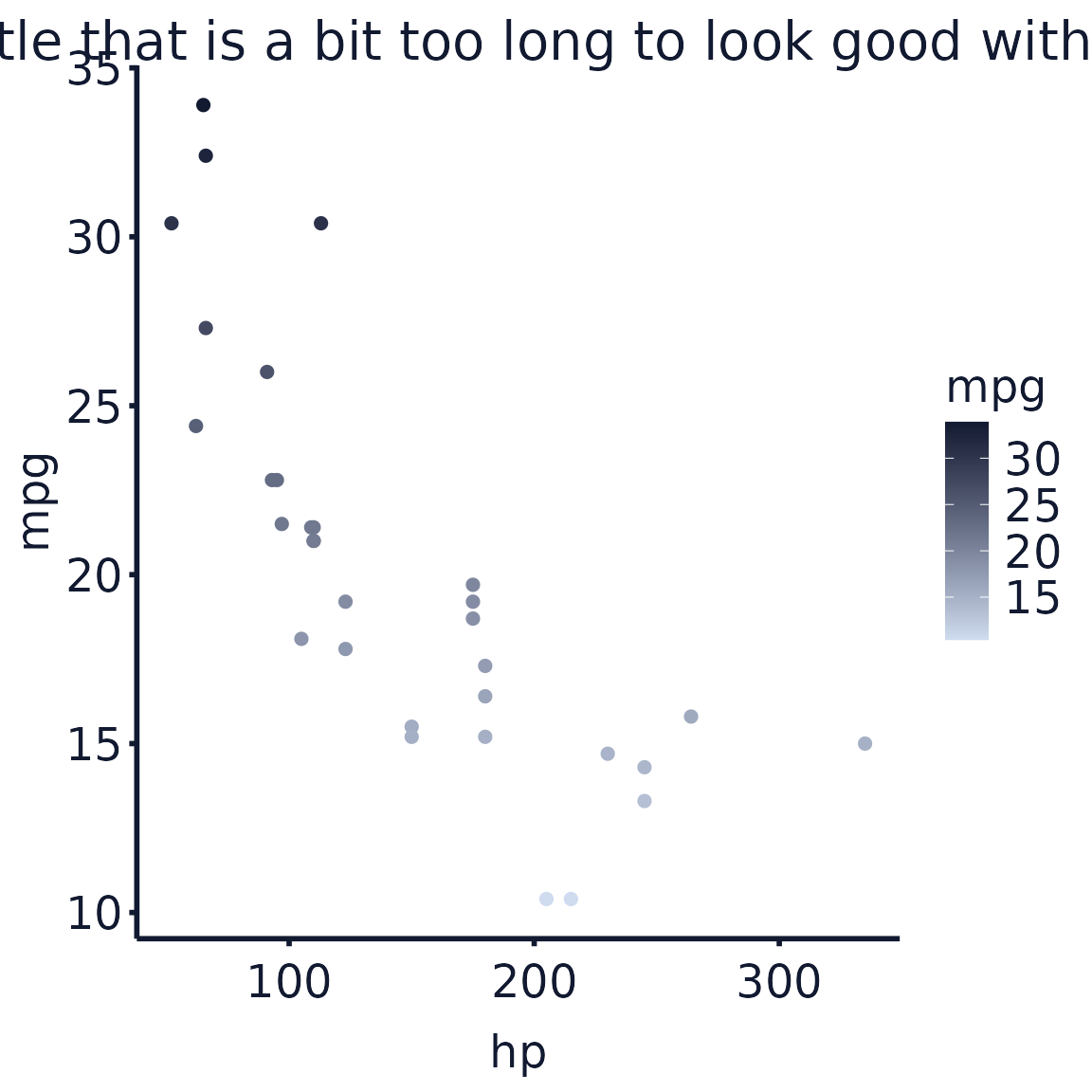

The title above gets cut off, but using text_wrapper() it will add a new line:

## add colour scheme and wrap text labels
cars_plot %>%
  exploristics_colour(colour_pal = "Expl_RGB") %>%
  text_wrapper()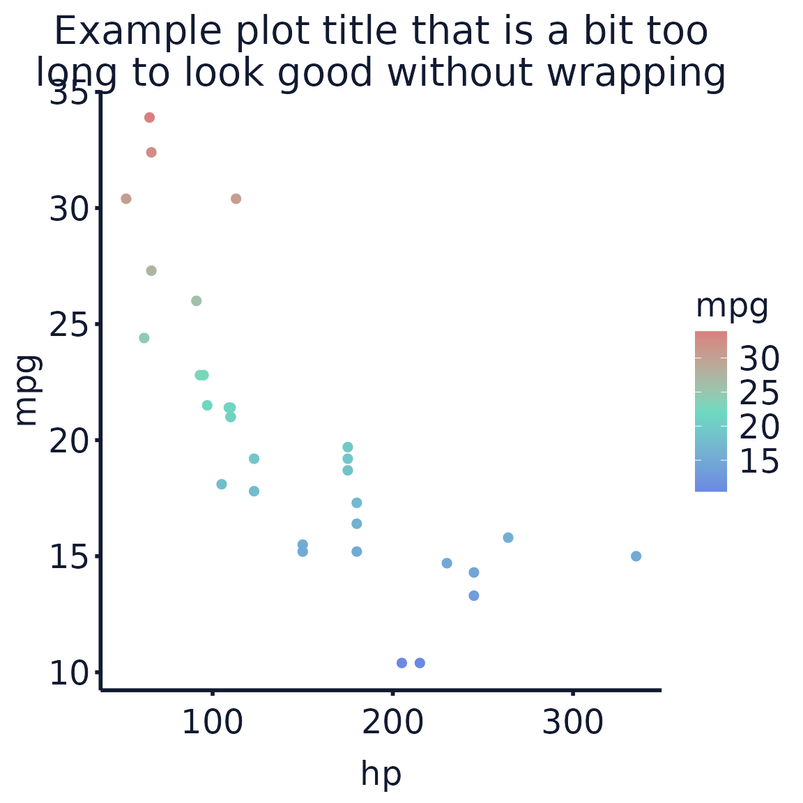

Save with logo

Adding to a ggplot

Use save_with_logo() to add a footer to your plot with the Exploristics logo and an optional text caption. Specify a filename without an extension to save the plot to. It will be saved with the footer added as a .png file.

## add colour scheme, wrap text labels and save with the Exploristics logo
cars_plot %>%
  exploristics_colour(colour_pal = "Expl_RGB") %>%
  text_wrapper() %>%
  save_with_logo(filename = "example_cars_plot", text = "Source:Data source\nProduced by: Name")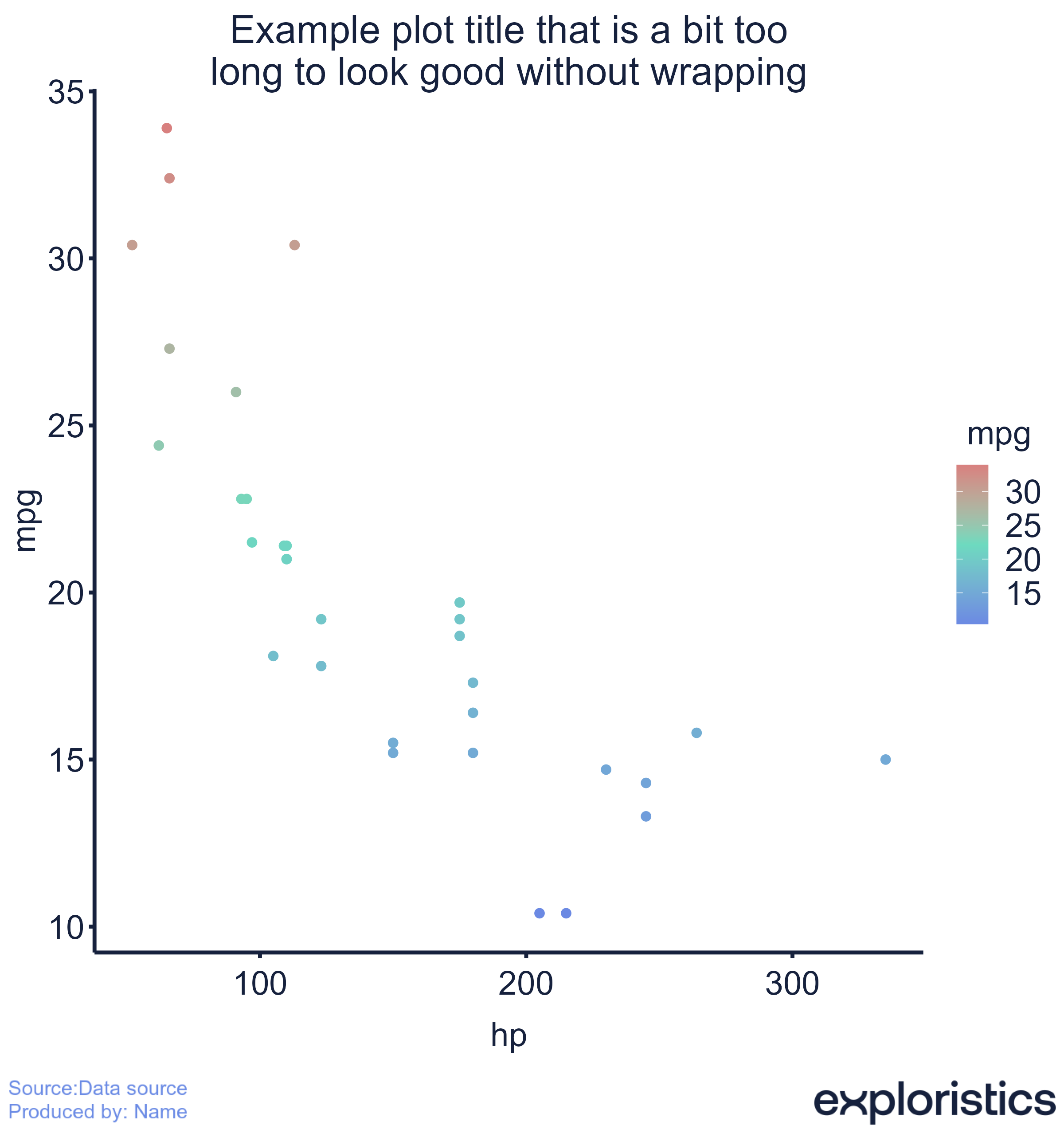

The saved plot with the footer added

Adding to an image

The footer can also be added to any image file. This could be a plot you’ve previously generated that didn’t use ggplot2. Here, a base R plot is saved to an image file. The file is then passed to save_with_logo() which will save a new plot with the footer added as a .png file. The default footer suffix of “_with_footer” is added so the original image file is not overwritten.

## create a plot and save to a file
png(
  filename = "example_cars_base_r_plot.png",
  width = 8,
  height = 5,
  units = "in",
  res = 300
)
plot(mtcars$hp, mtcars$mpg, pch = 19)
dev.off()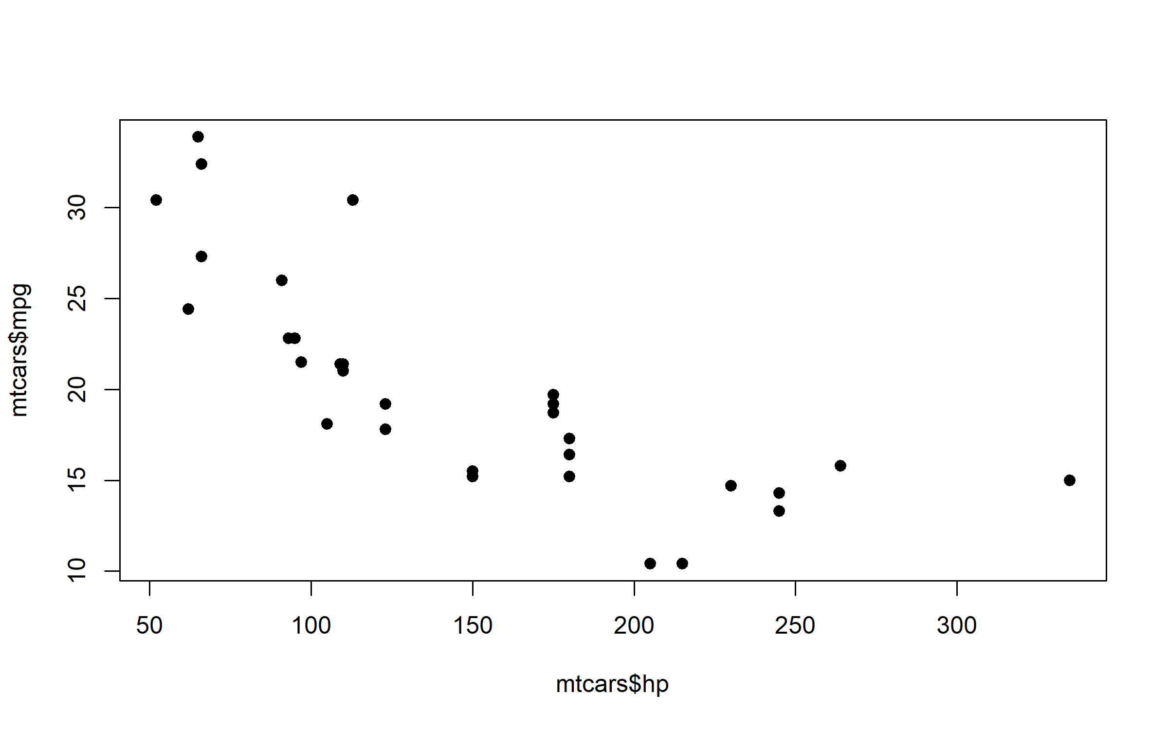

The image of the base R plot

## add the footer to the saved image with a custom caption
save_with_logo("example_cars_base_r_plot.png", text = "Source: Data source")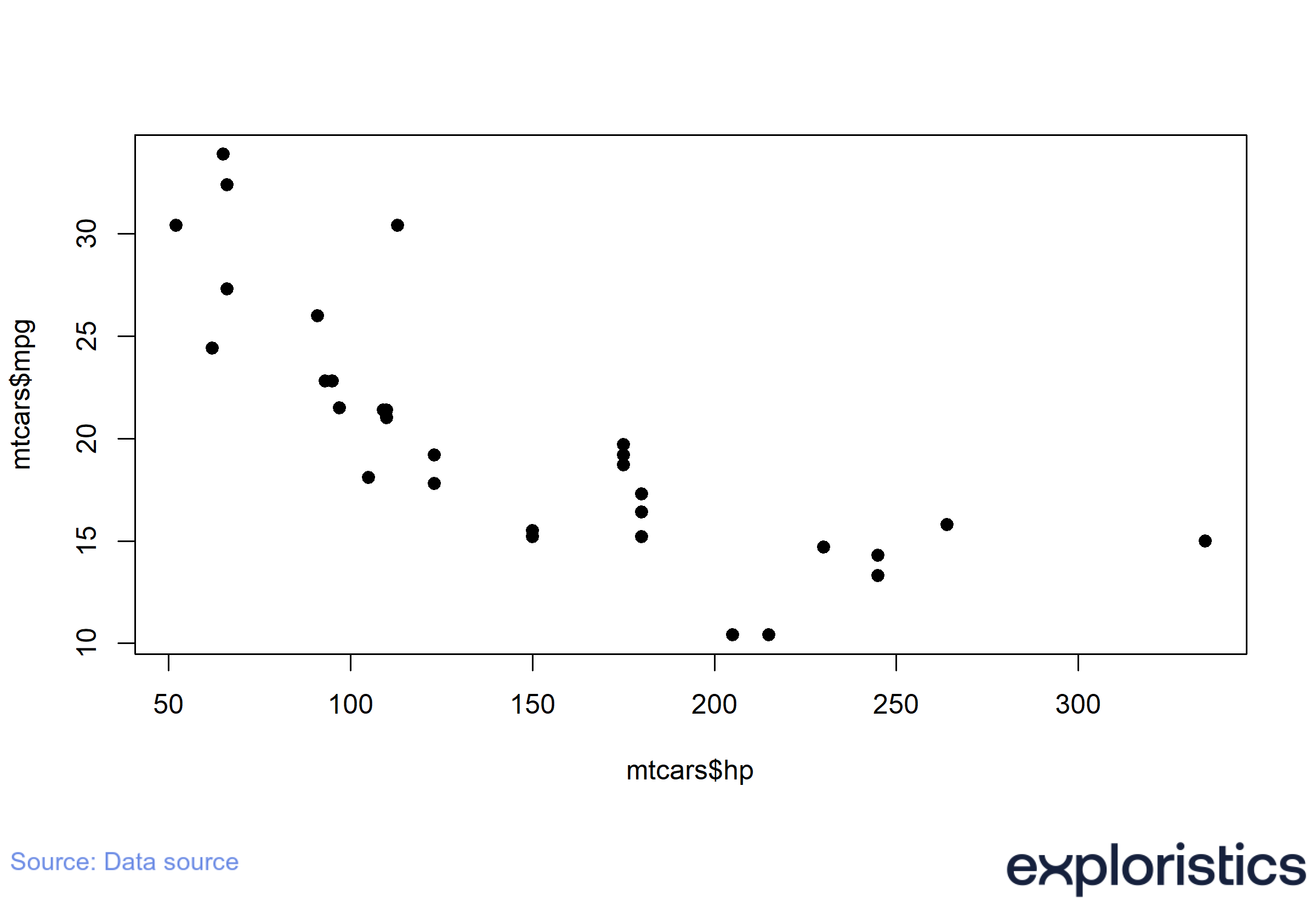

The same image with the footer added

Overwriting the default theme

If you want to change any option in the theme_exploristics() you can add another theme() call after it with the formatting you’d like to overwrite.

## generate a plot with the Exploristics theme
ggplot(data = mtcars, aes(x = hp, y = mpg, colour = mpg)) +
  geom_point(size = 2) +
  labs(title = "Example plot") +
  theme_exploristics()

## add `theme()` to change additional options or overwrite `theme_exploristics()` default values
ggplot(data = mtcars, aes(x = hp, y = mpg, colour = mpg)) +
  geom_point(size = 2) +
  labs(title = "Example plot") +
  theme_exploristics() +
  theme(legend.position = "top", legend.text = element_text(size = 12))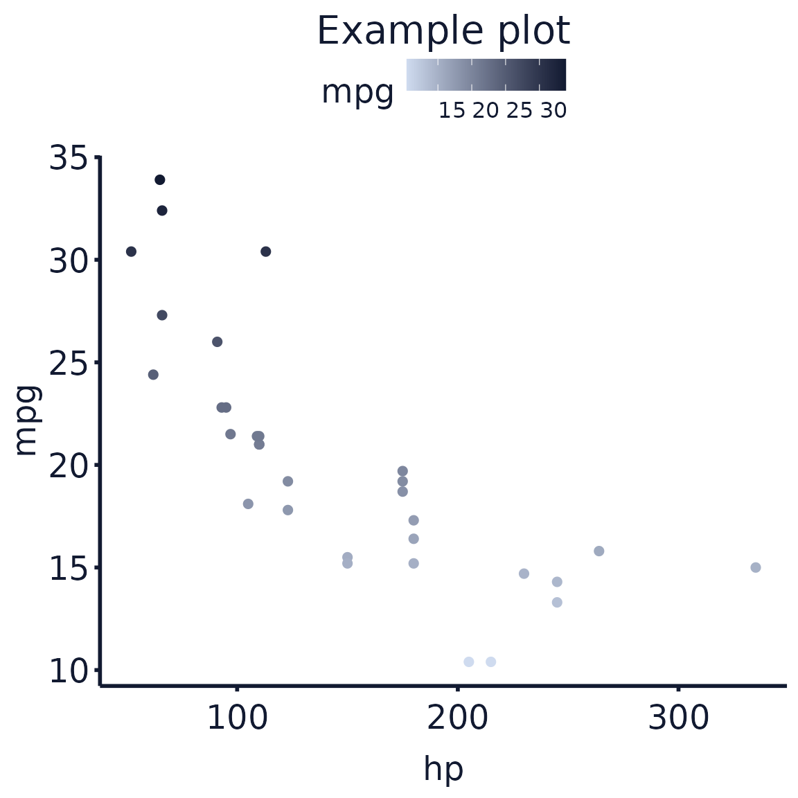

Removing function names from text label

In some cases you may want to plot variables as a specific class, e.g. a numeric variable as a factor. For this if you use text_wrapper() it will automatically clean the axis titles and legend titles to remove the as.*() functions applied when creating the plot.

## use a numeric variable as discrete by using `as.factor()` when setting `fill`
p <-
  ggplot(data = mtcars, aes(x = cyl, y = mpg, fill = as.factor(cyl))) +
  geom_bar(stat = "identity") +
  theme_exploristics()

## the legend title is "as.factor(cyl)"
p %>%
  exploristics_fill(colour_pal = "Expl_RGB")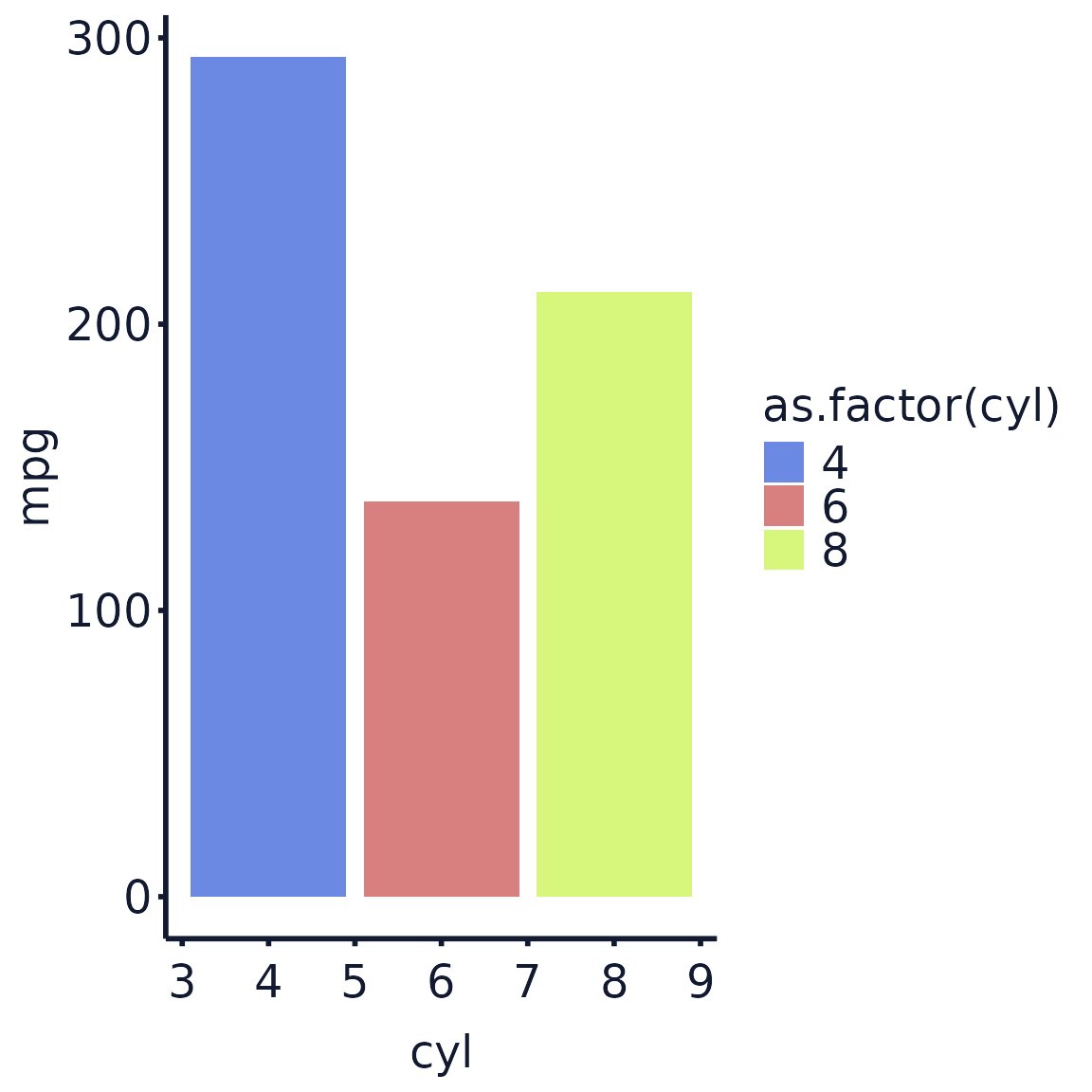

The legend title above would look better with the function call in it. Using text_wrapper() it will leave the legend title as just “cyl”:

## but using `text_wrapper()` the legend title is now "cyl"
p %>%
  exploristics_fill(colour_pal = "Expl_RGB") %>%
  text_wrapper()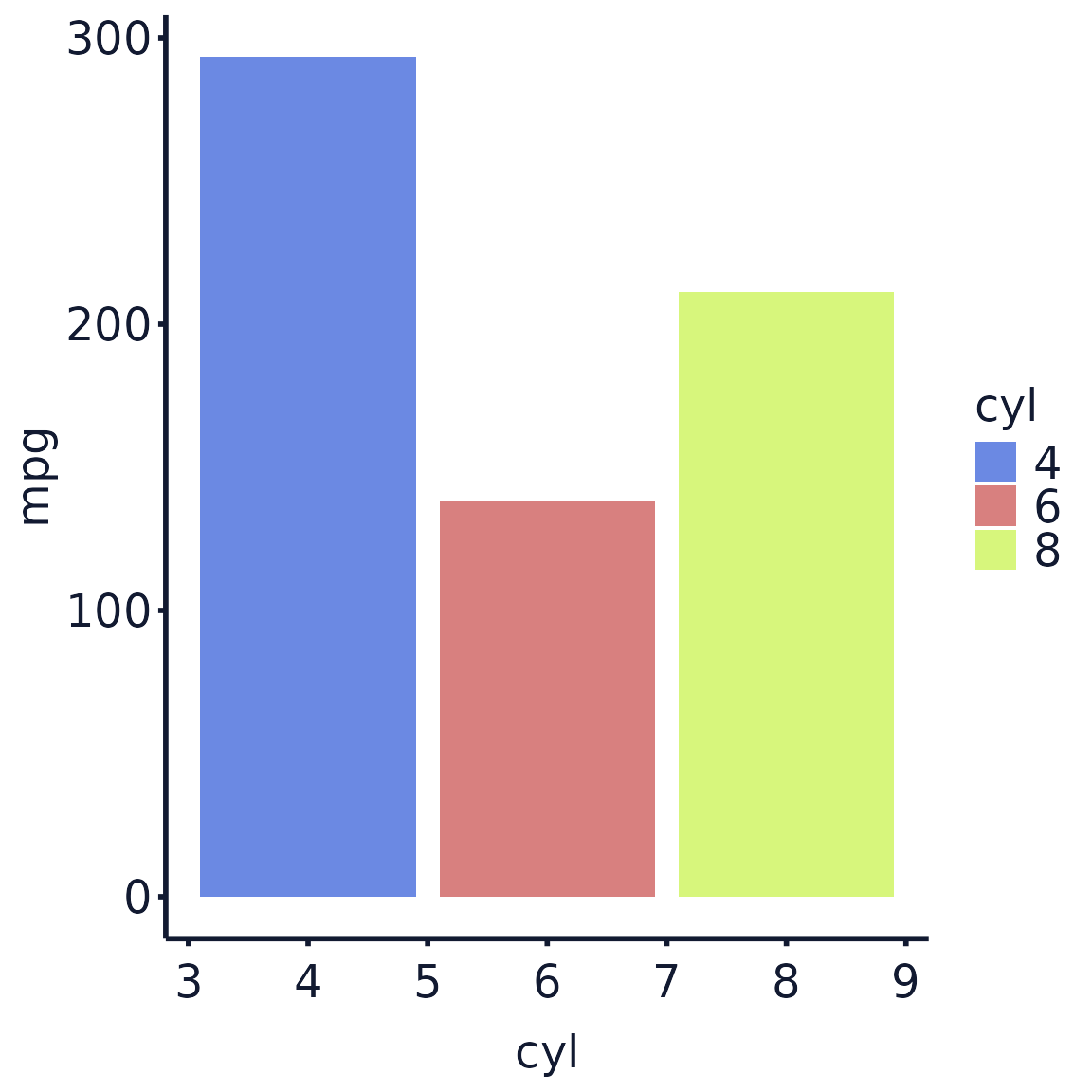

Potential issues

Using fill for bar plots

When setting fill and using geom_bar() the default border, which is set by colour, can cause horizontal lines to appear across the bars in the plot.

To fix this set fill and colour in aes() to the same variable and then add exploristics_fill() and exploristics_colour() with both using the same colour palette.

## barplot with both colour and fill specified
cars_plot_col_fill <-
  ggplot(data = mtcars, aes(
    x = cyl,
    y = mpg,
    fill = as.factor(cyl),
    colour = as.factor(cyl)
  )) +
  geom_bar(stat = "identity") +
  theme_exploristics()

cars_plot_col_fill %>%
  exploristics_fill(colour_pal = "Expl_RGB") %>%
  exploristics_colour(colour_pal = "Expl_RGB") %>%
  text_wrapper()

Amy McCorry